Mastering Excel Number Formatting: Display Values in K, M, B, and T with Custom Formats

Free downloadable cheat sheet Link at the end.....

📊 Formatting Numbers for Thousands, Millions, Billions & Trillions in Excel

Large numbers can quickly clutter your financial reports or dashboards. By scaling numbers into K (thousands), M (millions), B (billions), or T (trillions), you can create cleaner, more professional outputs for investors, clients, or internal stakeholders. These formats also pair beautifully with Excel functions like TEXT() for automated narratives.

We will use custom formatting to achieve exactly this.

🔢 Understanding Custom Number Format Structure

A custom number format in Excel follows this structure:​

Positive; Negative; Zero; Text

• Positive: Format for positive numbers

• Negative: Format for negative numbers

• Zero: Format for zero values

• Text: Format for text entries​

Each section is separated by a semicolon (;).

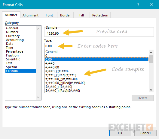
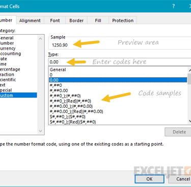
To apply custom formatting

1. Select the cell or range of cells you want to format.

2. Press Ctrl + 1 to open the Format Cells dialog box the below dialog box will appear

3. Finally select the Custom format from the sample codes after having previewed. Press OK.

🧱 Understanding Scaling with Commas in Custom Formats

Each comma removes three digits from the value shown.

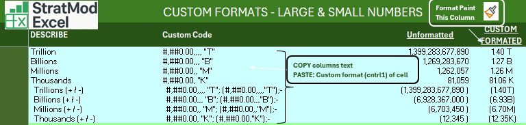
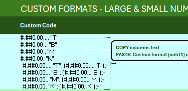
🔢 Custom Format Examples

🔹 1. Format in Thousands (K)

#,##0,"K"

Value Output

12,345 12K

-9,870 -10K

Add decimals: #,##0.0,"K" Displays: 12.3K

🔹 2. Format in Millions (M)

#,##0,, "M"

Value Output

3,450,000 3M

-1,850,000 -2M

Add decimals: #,##0.0,, "M" Displays: 3.5M

🔹 3. Format in Billions (B)

#,##0,,, "B"

Value Output

2,150,000,000 2B

-850,000,000 -1B

Add decimals: #,##0.0,,, "B" Displays: 2.2B

🔹 4. Format in Trillions (T)

#,##0,,,, "T"

Value Output

7,200,000,000,000 7T

-4,000,000,000,000 -4T

With decimals: #,##0.0,,,, "T" Displays: 7.2T

🎨 Formatting Negative vs Positive Values

To clearly differentiate negative and positive values, use color and symbols:

#,##0.0,, "M";[Red](#,##0.0,, "M")

Value Output

3,000,000 3.0M

-3,000,000 (3.0M) in red

You can apply this logic to any scale (K, M, B, T). For example, in billions:

#,##0.00,,, "B";[Red](#,##0.00,,, "B")

🧠 Using Custom Formats with TEXT(), CONCATENATE() & TEXTJOIN()

Custom number formats can be dynamically used in commentary strings or automated narratives using:

• TEXT() to apply the format

• CONCATENATE() or TEXTJOIN() to build dynamic text

📘 Example 1: Dynamic Commentary with TEXT + CONCATENATE

=CONCATENATE("Total revenue for Q1 is ", TEXT(A1, "#,##0.0,, 'M'"), ".")

If A1 = 3450000, the result is:

Total revenue for Q1 is 3.5M.

📘 Example 2: Narrative Using TEXTJOIN

=TEXTJOIN(" ", TRUE, "Our net loss was", TEXT(B1, "#,##0.0,, 'M'"), "due to increased costs.")

If B1 = -2750000, the result is:

Our net loss was -2.8M due to increased costs.

📘 Example 3: Positive/Negative Logic in Narrative

=IF(A1<0,

"We recorded a loss of "&TEXT(ABS(A1), "#,##0.0,, 'M'"),

"We made a profit of "&TEXT(A1, "#,##0.0,, 'M'")

)

If A1 = -4500000, output:

We recorded a loss of 4.5M

If A1 = 6200000, output:

We made a profit of 6.2M

✅ Summary Table of Format Strings

Smart Scaling with λLargeNumbers – One Function to Format Them All

As a final bonus in this guide, we're introducing an advanced Excel Lambda function that automates the formatting of large numbers into thousands (K), millions (M), billions (B), and trillions (T)—including both positive and negative values.

Instead of manually applying custom number formats or nesting IF() functions repeatedly, you can define a single dynamic and reusable Lambda called:

✅ λLargeNumbers

🔧 Lambda Definition:

=LAMBDA(Number,

IFS(

Number>=1000000000000,TEXT(Number,"#,##0.00,,,, ""T"""),

Number>=1000000000,TEXT(Number,"#,##0.00,,, ""B"""),

Number>=1000000,TEXT(Number,"#,##0.00,, ""M"""),

Number>=1000,TEXT(Number,"#,##0.00, ""K"""),

Number<=-1000000000000,TEXT(Number,"(#,##0.00,,,,""T"")"),

Number<=-1000000000,TEXT(Number,"(#,##0.00,,,""B"")"),

Number<=-1000000,TEXT(Number,"(#,##0.00,,""M"")"),

Number<=-1000,TEXT(Number,"(#,##0.00,""K"")"),

TRUE,TEXT(Number,"#,##0;(#,##0);-")

))

💡 How It Works:

• IFS() checks the size of the number and applies the correct formatting scale.

• TEXT() applies Excel's custom number format.

• Negative values are automatically wrapped in brackets using the relevant custom format.

• Values under 1,000 fall back to a default readable format: #,##0;(#,##0);-

📊 Example Use Case

Input Value Output

=λLargeNumbers(1234) 1.23K

=λLargeNumbers(2300000) 2.30M

=λLargeNumbers(-1570000000) (1.57B)

=λLargeNumbers(0) -

💼 Perfect for:

• Dashboards

• Investor decks

• Commentary generation

• Financial modeling summaries

Investor decks

• Commentary generation

• Financial modeling summaries

🔄 Pro Tip: Pair With TEXTJOIN or CONCAT

=TEXTJOIN(" ", TRUE, "Q2 profit was", λLargeNumbers(B2))

→ Q2 profit was 2.45M

=CONCATENATE("Cash burn: ", λLargeNumbers(C5))

→ Cash burn: (1.08M)

📥 Download the Cheat Sheet: To make your formatting faster and more consistent, we’ve compiled all large number formats, including this Lambda logic, into a free downloadable cheat sheet.