Excel Power Query vs LAMBDA vs VBA for Unpivoting Data

In any Excel model, getting the data layout right is basically everything.

When it’s wrong, Excel sort of penalizes you for it. Stuff that should be easy gets weirdly hard. Lookups become messy. Calculations sprawl all over the place. PivotTables stop being fun and start being a “why is this not working” situation.

And the biggest offender is usually the same thing.

That cross tab layout.

You know the one. Categories down the left. Dates or months across the top. Values scattered across a grid. It looks tidy to the eye, sure. But it’s a pain to work with.

What you actually want, especially if you’re building models, is the list layout (also called data layout). One column for the values. The categories stay as columns. Every record is a row.

So the process of shifting from cross tab to list layout is called unpivoting.

The video this post is based on shows four quick ways to unpivot in Excel: Power Query, a custom VBA function, a LAMBDA function (the creator’s favorite), and a formulas only method that also works well.

All 4 work. The question is which fits your situation. Download the Example File to follow along.

First, what unpivoting actually fixes (and why it matters)

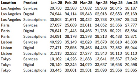
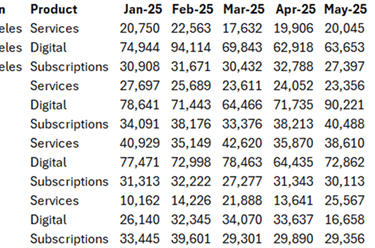
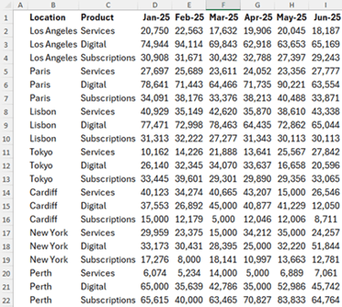
If your data is laid out like this:

● Location in rows

● Product in rows

● Dates or periods across columns (Jan, Feb, Mar… or actual dates)

● Values inside the grid

That’s a cross tab.

And it causes two big problems:

1. It’s harder to do calculations and lookups because values are spread across many columns instead of one.

2. It’s essentially unusable for PivotTables and proper data modeling (because PivotTables and models want a single “Amount” column with a “Date” column next to it).

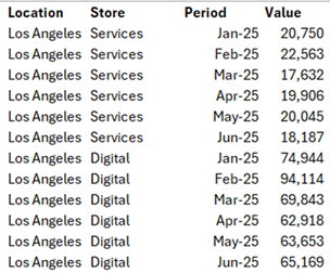
When you unpivot it, you get something like:

That’s the list layout.

Now everything gets easier. PivotTables. Lookups. Power Pivot. Measures. Even just filtering properly.

So yeah. Unpivoting is not a fancy trick. It’s one of those “your future self will thank you” moves.

Method 1: Power Query (fast, clean, but refresh driven)

Power Query is the most “official” feeling way to unpivot in Excel. It’s built for this.

How the Power Query unpivot works

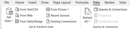
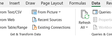
1. Select any cell in your table.

2. Go to Data tab.

3. Click From Table/Range.

4. Power Query opens and detects your table. Click OK.

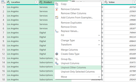
5. Select your category columns (in the video example it’s the first two columns, like Location and Product).

6. Right click and choose Unpivot Other Columns.

7. Choose your load option. You can:

○ load as a table

○ load to the data model (the video creator likes this)

○ load to an existing worksheet location

Done. Your cross tab becomes a list.

Then the video points out a final cleanup step that’s important:

● Check data types.

● Text columns are fine as text.

● Date columns might need conversion to Date.

● Amount is usually a whole number (or decimal), set it appropriately.

Power Query then outputs your unpivoted table.

What’s good about Power Query

● Very reliable.

● Very repeatable once set up.

● Handles big data nicely.

● The steps are visible. You can audit them.

● Great if you’re pulling data from files, folders, databases.

The big drawback

If you have multiple tables to unpivot, you often end up building a query per table, and you have to remember to refresh.

That refresh part is the “ugh” for some models. Especially if what you really want is a simple function, something you can type like a formula and it updates automatically.

Which leads to the next two methods.

Method 2: VBA function (formula like convenience, but it’s VBA)

The video creator built a custom VBA function for unpivoting. Basically, you type it like a formula, it spills the results, and you’re done.

How you use it

You type:

=vUNPIVOT(range, static_columns)

The creator named it with a V at the front on purpose. Because maybe one day Microsoft releases an UNPIVOT function, and this avoids name conflicts.

It takes two inputs:

1. The range of the cross tab.

2. The number of static columns (the columns you want to keep as category columns).

Example in the video:

● Static columns are Location and Product

● So static columns = 2

So you use:

● range = the whole table

● static = 2

And it spills out the unpivoted list.

The part that’s genuinely nice

The VBA function has auto-trimming.

So if you extend your selected range to be more “scalable” like:

● extend to 100 rows even if your data only uses 20

● extend to extra columns beyond what’s populated

It automatically removes the empty rows and keeps the output neat.

That’s a big deal in real models because people love to oversize ranges “just in case”, and then you get a bunch of zeros and junk. VBA can clean that up.

How to install it (as shown)

● Make sure you have the Developer tab enabled.

○ Right click the ribbon

○ Customize ribbon

○ Tick Developer

● Go to Developer > Visual Basic

● Insert a Module

● Paste the code for the function into the module

The video mentions you can grab the code from the provided exercise file download. And you don’t need to understand the VBA, just install it.

Pros of the VBA method

● Works like a formula (simple inputs).

● No Power Query setup.

● No refresh step.

● Auto trims empty rows and columns (in the creator’s function).

● Easy to reuse across multiple tables without building separate queries.

The drawback (and it’s a real one)

It requires macros.

And macros are still a deal breaker in many environments:

● People don’t want to enable them.

● Web sharing is messy.

● Some companies block them.

● Macro-enabled files can’t always be used the way you want.

So the video moves to the next method, which keeps the “formula-like” experience, but without VBA.

Method 3: LAMBDA function (the favorite, no macros, still formula driven)

This is the creator’s preferred method. And honestly, it makes sense.

You get:

1. the simplicity of a function

2. no refresh

3. no VBA

4. works in non macro workbooks

5. better for sharing and collaborating (including web scenarios)

How you use it

The function name used in the video is:

XUNPIVOT

Same naming logic as before. X prefix avoids future naming collisions if Microsoft ever ships UNPIVOT as a native function.

Usage looks like:

=XUNPIVOT(range, static_columns)

Same two arguments:

1. range

2. number of static columns (Location + Product = 2 in the example)

And it spills the list output.

The one “gotcha” compared to the VBA function

If you extend the range bigger than your data (like taking it to 100 rows), the LAMBDA version initially returns extra zeros at the bottom.

It doesn’t auto trim by default.

But the creator added a simple feature: you can trim the range using a dot.

So you basically append a dot to trigger trimming, and it removes the extra zeros / blank output.

In the video they show:

● extend range down, see zeros

● add the dot trim symbol

● zeros disappear

● extend columns too, still trimmed

So you get the same scalability idea, just with an extra step if you’re oversizing your input range.

How to install the LAMBDA

THE FORMULA - =xUnpivot

=LAMBDA(dataRange,[staticCols],

LET(

sc, IF(ISOMITTED(staticCols), 1, staticCols),

headers, DROP(INDEX(dataRange, 1, ), , sc),

dataRows, DROP(dataRange, 1),

rowCount, ROWS(dataRows),

colCount, COLUMNS(headers),

totalRows, rowCount * colCount,

result,

MAKEARRAY(

totalRows,

sc + 2,

LAMBDA(i,j,

LET(

r, INT((i - 1) / colCount) + 1,

c, MOD(i - 1, colCount) + 1,

IF(j <= sc,

INDEX(dataRows, r, j),

IF(j = sc + 1,

INDEX(headers, c),

INDEX(dataRows, r, sc + c)

))))),

result))

Because LAMBDA is stored as a named formula:

● Go to Name Manager

● Create a new name

● Name it XUNPIVOT (or whatever you want)

● Paste the LAMBDA formula definition in

Again, the video says it’s in the downloadable exercise file, so you don’t have to build it from scratch.

Why this method is such a sweet spot

● It behaves like a formula.

● It works in standard .xlsx (no macros).

● It’s share friendly.

● You can reuse it quickly across sheets and models.

● You don’t have to keep building Power Query queries.

The creator even says, basically, this is tremendous. Preferred.

But then they point out one more thing.

If you lose the LAMBDA definition. Or lose the VBA module. Or you’re in a workbook where neither is available. And you also don’t want to set up Power Query.

You still might want to know how to do it with regular formulas.

Which brings us to the final method.

Method 4: Formulas only unpivot (no PQ, no VBA, no LAMBDA… just Excel)

The solution uses three formula areas:

● One formula that creates the “Value” column by combining multiple columns into one using a method similar to this TOCOL type function

● A formula approach for the row labels output

● A formula approach for the column labels output (like Date)

The “Value column” logic, uses a TOCOL type function to combine multiple columns into a single column.

That combined result then feeds the other formulas (one for rows and one for columns).

The case study – we are seeking to unpivot the data in cells B1:I22.

1. The Core: The "Values" Column (Column P)

The engine of this transformation is the TOCOL function, which is responsible for collapsing the 2D grid of values into a single vertical list.

• Formula: =TOCOL(D2:I22, 1)

• How it works: This function scans the monthly data (Jan-25 through Jun-25) row by row. The second argument, "1", tells Excel to ignore any blanks in the range. This ensures that if your range is extended for scalability, the final list remains "austere" and free of unnecessary zeros.

• Result: This creates a spilled range in cell P2#. Because the other formulas for rows and periods rely on the size of this list, it is essential to write this formula first.

2. The "Period" Labels (Column O)

Once the values are listed, you need to assign the correct date (Column Header) to each value. This is achieved by cycling through the headers repeatedly.

• Formula: =INDEX(D1:I1, MOD(SEQUENCE(ROWS(P2#), 1, 0), COLUMNS(D1:I1)) + 1)

• The Logic:

◦ SEQUENCE(ROWS(P2#), 1, 0): This creates a list of numbers starting from 0, as long as your unpivoted value list.

◦ MOD(..., COLUMNS(D1:I1)): The MOD function divides those sequence numbers by the number of months (6) and returns the remainder. This causes the count to "reset" (0, 1, 2, 3, 4, 5, 0, 1...) every 6 rows.

◦ INDEX: This uses that repeating count to grab the header (Jan, Feb, Mar...) over and over again for every row in the new list.

3. The "Row Field" Labels (Columns M & N)

Finally, you must repeat the static category labels (Location and Product) for every associated value. Unlike the Period labels that cycle, these must stay the same for a set number of rows before moving to the next category.

• Formula (for Location): =INDEX(B2:B22, ROUNDUP(SEQUENCE(ROWS($P$2#)) / COLUMNS($D$1:$I$1), 0))

• The Logic:

◦ SEQUENCE(ROWS($P$2#)): Again, this creates a list of numbers (1, 2, 3...) based on the total number of unpivoted values.

◦ / COLUMNS($D$1:$I$1): This divides the sequence by 6 (the number of months).

◦ ROUNDUP(..., 0): This ensures that for the first 6 values, the result is "1"; for the next 6, it is "2", and so on.

◦ INDEX: This tells Excel to stay on the first Location ("Los Angeles") for 6 rows, then move to the second Location ("Paris") for the next 6.

So you end up with the same unpivoted list layout as:

● VBA function

● LAMBDA function

● Power Query

When formulas are actually useful

This method is great when:

● You cannot use macros.

● You don’t want Power Query (or it’s blocked, or you’re keeping the model lightweight).

● You don’t have the custom LAMBDA function saved.

● You want everything visible in cells and auditable.

But it’s also the method that tends to be the most… fragile. Not wrong, just easier to break if someone unexpectedly edits the structure. And it can be more effort to set up the first time.

Still, it’s a real option. And it’s nice to know it’s there.

So which one should you use? (honest comparison)

Here’s the practical comparison, based on what the video highlights.

Power Query is best when

● You’re working with external data sources.

● You want a clean ETL workflow (import, transform, load).

● You expect to refresh data periodically and that’s acceptable.

● You like seeing transformation steps.

But if you have many separate tables and just want quick formula style unpivoting, building and refreshing many queries gets old.

VBA function is best when

● You want a simple function call.

● You want auto trimming behavior.

● You control the environment (macros allowed).

● You’re building internal tools where .xlsm is fine.

But if you’re sharing with macro hesitant users, this becomes a blocker fast.

LAMBDA function is best when

● You want a function-like experience without macros.

● You want it to work in normal workbooks.

● You want something reusable and share friendly.

The only real drawback from the video is that trimming isn’t automatic unless you use the creator’s dot trim feature.

Still, for most modern Excel users, this is probably the best balance.

Formulas only is best when

● You need a “works anywhere” solution.

● You can’t rely on custom functions being installed.

● You’re okay with more complex cell logic.

It’s the most portable approach in a weird way. Because it’s just formulas. But it’s also the least elegant to maintain unless you package it nicely.

FAQ

What does “unpivot” mean in Excel?

Unpivoting converts a cross-tab layout (values spread across many columns) into a list layout where those column headers become a single column (like Date), and the values go into one Value or Amount column.

Why can’t I create a PivotTable from a cross tab layout?

PivotTables work best with normalized list data. Cross tabs often confuse the structure because you don’t have a single field for things like Date or Period; you have many separate columns instead.

Is Power Query the easiest way to unpivot?

For a single table, yes. Select table, open Power Query, pick “Unpivot Other Columns”, and load back. Very fast. The main downside is managing refresh and multiple queries if you have lots of tables.

What’s the advantage of using a VBA unpivot function?

It behaves like a formula. No Power Query steps, no refresh, and in the video’s function it also auto-trims empty rows and columns when you oversize the input range.

Why would I avoid VBA for unpivoting?

Because it requires macros. Many users and organizations block macros or dislike enabling them, and macro-enabled files can be awkward for web based collaboration.

What’s the advantage of using a LAMBDA unpivot function?

It gives you the formula-like experience without macros. You can use it in non-macro workbooks and share it more easily. In the video, this is the creator’s preferred method.

Why does the LAMBDA method sometimes show zeros at the bottom?

If you oversize your input range (like selecting 100 rows when only 20 have data), the LAMBDA output may include empty results as zeros. The creator solves this by adding a trimming option using a dot.

Can I unpivot using only Excel formulas?

Yes. The video shows a formulas-only solution using a combined values approach (like TOCOL) plus supporting formulas for the other columns. It’s more complex to build, but it works without Power Query, VBA, or custom LAMBDAs.

Which unpivot method is best for sharing a workbook with others?

Usually, the LAMBDA method, because it avoids macros. Power Query is also shareable, but users may need to refresh and have the same query setup. VBA is the least share-friendly if macros are restricted.

Do these methods work equally well?

For a single table, yes. The video’s point is that all four methods can unpivot successfully. The differences are mostly around setup time, portability, refresh behavior, and whether macros are allowed.