Smarter Budget Variance Analysis in Excel: Custom Formats with Arrows, Symbols & Color

Bonus download at the end.......

Ditch Conditional Formatting: Smarter Excel Variance Visuals with Custom Formats

When it comes to budget variance analysis, Excel Conditional Formatting is a familiar go-to. But there's a smarter, leaner, and more scalable way to bring clarity to your deviations—Custom Number Formats.

This guide introduces a powerful combination of techniques:

• UniChar & Symbols

• Font Color within Formats

• Positive, Negative, Zero logic

• Bonus: 3-Scale & 4-Scale Conditional Logic using Formulas

Instead of relying on Conditional Formatting rules for every cell, you can hardwire logic into the cell's display using Excel's Custom Format Brackets and formulas.

⚡ Why Custom Formats are Faster than Conditional Formatting

While both Custom Number Formatting and Conditional Formatting improve Excel’s visual clarity, they work very differently under the hood—and that difference can drastically affect performance, especially in larger workbooks.

🧠 Custom Formats: Fast by Design

Custom number formats are display-only rules. They simply tell Excel how to render the value in each cell. Once applied, they don’t need to evaluate logic or respond to cell-by-cell changes dynamically. This makes them:

• Lightweight

• Memory-efficient

• Highly scalable for large datasets

🧨 Conditional Formatting: Logic-Heavy

In contrast, conditional formatting applies formulas or rules to each cell individually. Every time a value changes—or when the file recalculates—Excel re-evaluates the rules for each affected cell. This causes:

• Slower recalculation times

• Heavier processor load

• Noticeable lags in large sheets

📊 Benchmark Results from Leading Excel Experts

✅ Conclusion: When performance matters—especially with dashboards or large financial models—custom number formats are the smart choice.

🧠 Why Use Custom Formats Over Conditional Formatting?

✅ No extra formatting rules

✅ Lighter, faster spreadsheets

✅ Works natively with copy-paste and pivot tables

✅ Visuals remain consistent even when Conditional Formatting breaks

🔢 Understanding Excel's Custom Format Structure

The syntax follows:

[Positive Format];[Negative Format];[Zero Format];[Text Format]

Yes—you can format text too!

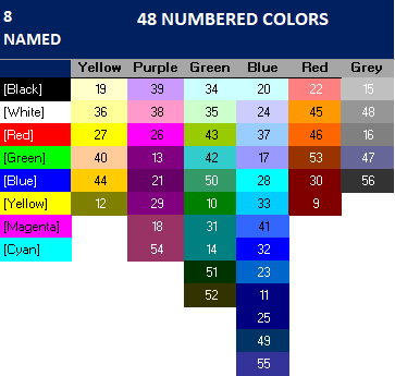
🟦Excel’s 56-Color Palette—Add Visual Flair to Formats

You can apply colors directly in number formats using Excel’s legacy 56-color palette.

🟦 Syntax:

[ColorX]#,##0

Where X is a number from 1 to 56.

🔹 Example:

[Color10]#,##0;[Color3](#,##0);[Color16]"–"

Download the full Excel color palette guide: 📥 Excel 56 Color Cheat Sheet (Free Download).

🔣 Using UNICHAR Symbols in Custom Formats

Excel's UNICHAR() function unlocks a world of visual possibilities by allowing you to insert Unicode characters—such as arrows, ticks, emojis, and trend icons—directly into your cell displays.

While UNICHAR is commonly used in formulas (e.g. =UNICHAR(9650) for an ▲), you can hardcode the character into custom number formats as a text string. This lets you replace numeric or text values with highly visual icons, improving readability and impact in dashboards or variance tables.

✅ Commonly Used Unicode Characters

Here are just a few examples of what you can do:

You can use these characters in custom formats like so:
[Color10]"▲";[Red]"▼";"-"
or
[Color10]"✔"#,##0;[Red]"✕"#,##0;"-"

🌐 Explore the Full Unicode Library

If you're looking for more characters to experiment with, check out this comprehensive Unicode reference:
🔗 Copy and Paste Bullet Points, Symbols, and Characters | Bizuns

Just copy the character you like and paste it into your format string (inside quotes).

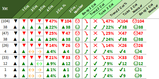
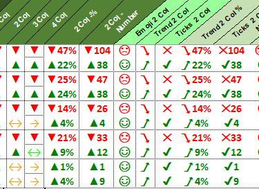
🧩 Format Recipes for Budget Variance Analysis

Each of these formats uses a combination of Unicode symbols, color codes, and Excel's native format logic.

💡 These work especially well in variance tables, dashboards, and management packs.

🎯 Bonus: Formula-Based 3-Scale & 4-Scale Logic

For nuanced variance grading, pair formulas with the custom formats.

✅ 3-Scale Scoring Formula (Positive / Neutral / Negative)

=LET(

Number, AC6,

IFS(Number > 5%, 1,

Number > 0, 0,

TRUE, -1)

)

Use these formulas in a helper column, and apply a custom format like:

[Color10]"▲";[Red]"▼";[Color45]"↔";"-"

✅ 4-Scale Scoring Formula (High / Moderate / Low / Negative)

=LET(

Number, AC16,

IFS(Number >= 10%, 1,

AND(Number > 5%, Number < 10%), 0,

Number > 0, "t",

TRUE, -1)

)

Use these formulas in a helper column, and apply a custom format like:

[Color10]"▲";[Red]"▼";[Green]"↔";[Color45]"↔"

Want to try all these formats instantly?

👉 Download the Custom Format Cheat Sheet (Ready to Copy & Paste)

It includes:

• Copy-ready format codes

• Example data tables

• Pre-written formulas

• Notes on customization