Most standard loan amortization tables in Excel work perfectly—until real-world complications arise. Please feel free to download our free Excel dynamic loan amortization schedule from one of our previous articles as an example.

When interest rates fluctuate or you need to account for balloon payments, traditional static models break down and require extensive manual adjustments.

Dynamic loan amortization solves this challenge by creating self-adjusting schedules that automatically adapt to changing conditions. This approach is essential for:

• Financial modeling accuracy when rates vary over the loan term

• Real-world lending scenarios, including access bonds with deposits and withdrawals

• Portfolio management where multiple rate changes occur

• Professional financial analysis requiring flexible, scalable solutions

Please download the Advanced Loan Amortization Template to follow along.

This comprehensive guide walks you through building an advanced Excel loan amortization model that handles:

• Multiple interest rate changes across different date intervals

• Automatic recalculation when any input parameter changes

• Balloon payments and lump sum transactions

• Visual indicators for rate change periods

By the end, you'll have a fully dynamic template that eliminates manual formula adjustments and adapts instantly to any loan scenario you encounter.

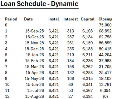
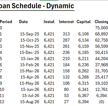
Understanding Loan Amortization Basics in Excel

Before diving into advanced techniques for building an advanced loan schedule in Excel, establishing a solid foundation with basic loan amortization components is essential. Every Excel financial modeling loan repayment schedule starts with four fundamental inputs that drive all subsequent calculations.

Core Input Requirements

• Start Date – The initial date when the loan begins

• Loan Period – Total duration of the loan (typically expressed in months)

• Interest Rate – Annual %rate charged on the outstanding balance

• Principal Amount – The initial capital borrowed

Standard Column Structure

These inputs generate 6 columns that form the backbone a amortization table:

• Period Number – Sequential numbering starting from zero

• Installment Date – The due date for each payment

• Opening Balance – Outstanding loan amount at the start of each period

• Interest Portion – Amount of each payment allocated to interest charges

• Principal Portion – Amount of each payment reducing the loan balance

• Closing Balance – Remaining loan balance after each payment

Essential Excel Functions

Building these calculations requires mastery of five key functions:

• SEQUENCE – Generates consecutive period numbers automatically

• EDATE – Calculates installment dates by adding months to the start date

• PMT– Computes the total monthly payment amount

• IPMT – Isolates the interest component of each payment

• PPMT – Extracts the principal repayment portion

1. Modeling Variable Interest Rates Dynamically

Standard loan tables break when interest rates fluctuate. A fixed-rate Excel loan model with rate changes step by step requires rebuilding formulas manually each time rates adjust—an inefficient approach for real-world scenarios where central banks regularly modify lending rates.

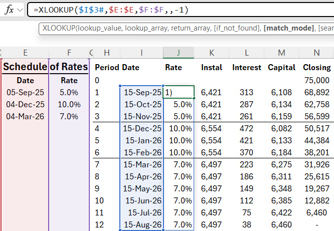
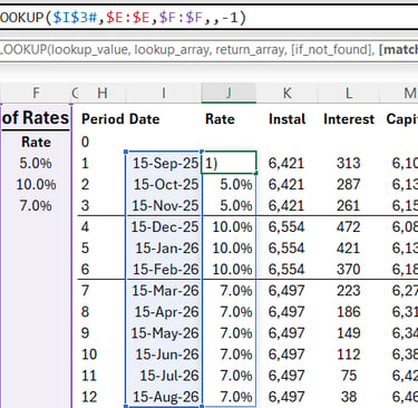
Building a Multi-Rate Schedule

The foundation of advanced loan amortization excel starts with a separate interest rate schedule containing:

• Effective dates - When each new rate takes effect

• Rate percentages - The applicable interest rate for each period

• Date intervals - Clear boundaries between rate changes

For example, a schedule might show 5% from September 5 to December 4, 10% from December 4 to March 4, and 7% thereafter.

Dynamic Rate Assignment with XLOOKUP

The XLOOKUP function solves the rate-matching challenge through its non-exact match mode. The formula structure:

=XLOOKUP(date_column, rate_schedule_dates, rate_percentages, , -1)

The -1 match mode parameter enables ascending non-exact lookup, which returns the most recent rate applicable to each installment date. When the function encounters a date between intervals, it automatically selects the correct rate from the preceding period.

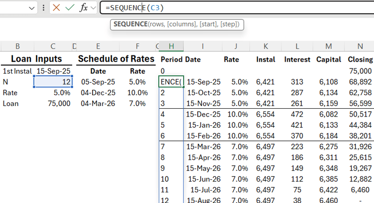
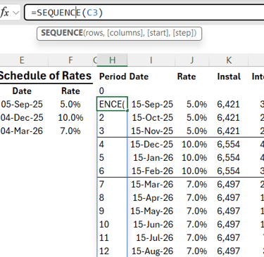
Period Numbering with SEQUENCE

The SEQUENCE function generates consecutive period numbers automatically:

=SEQUENCE(loan_period)

This creates a dynamic counter from 0 through the total loan term, eliminating manual numbering and enabling the schedule to expand or contract based on input changes.

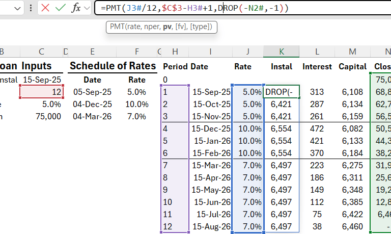
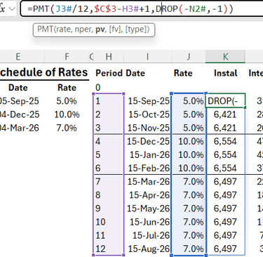
2. Calculating Installments & Balances with Changing Rates

With the dynamic interest rate structure in place, the next step involves calculating accurate payment amounts and tracking balances throughout the loan term. The PMT function serves as the foundation for determining monthly installments, but requires careful adjustment to account for variable rates.

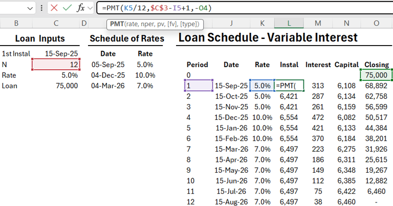
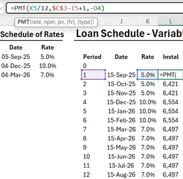
Breaking Down the PMT Calculation

The installment formula adapts to each period's specific circumstances:

excel =PMT(Rate/12, RemainingPeriod, -Capital)

Key components:

• Rate/12: Divides the annual interest rate by 12 for monthly calculations

• Remaining Period: Total loan period minus current period number, plus one to balance the calculation

• Negative Capital: The opening balance must be negative to return a positive payment amount

Splitting Payments into Components

Each installment consists of two distinct portions that shift as the loan progresses:

Interest Component: excel =(Rate/12) * OpeningBalance

Principal Component: excel =Installment - Interest

This separation reveals how much actually reduces the debt versus what covers borrowing costs. As rates fluctuate, the interest portion adjusts automatically while the principal repayment compensates to maintain consistent installments.

Tracking Balance Movements

The closing balance calculation follows a straightforward pattern:

excel =OpeningBalance - PrincipalPortion

Each period's closing balance becomes the next period's opening balance, creating a cascading effect that accurately reflects principal repayments across the entire schedule. This approach ensures the excel amortization schedule dynamic array formulas maintain accuracy even when interest rates shift multiple times throughout the loan term.

To manage these calculations effectively, employing financial functions in Excel can be immensely beneficial. Learning how to create a debt schedule using these functions will provide a structured approach to track your loans and their evolving balances accurately.

A More Automated Solution

If you’d prefer a ready-made model that consolidates multiple loans with variable interest rates and generates automated amortization schedules, check out the Excel Variable Rate Loan Portfolio Tool (1–1,000+ loans in one model).

3. Making the Loan Schedule Fully Dynamic & Self-Adjusting

Static loan tables present a significant challenge when you need to extend the loan period or modify input parameters. Each change requires manually dragging formulas down or adjusting cell references—a time-consuming process prone to errors in advanced excel functions for loan modeling.

Enabling Iterative Calculations

Before transforming your table into a dynamic excel loan template with balloon and lump sum capabilities, you must configure Excel's calculation settings:

1. Navigate to File > Options > Formulas

2. Locate the Iterative Calculations section

3. Check the box to Enable iterative calculation

This setting allows Excel to handle circular references and self-adjusting ranges that dynamic arrays require.

Implementing Dynamic Array Techniques

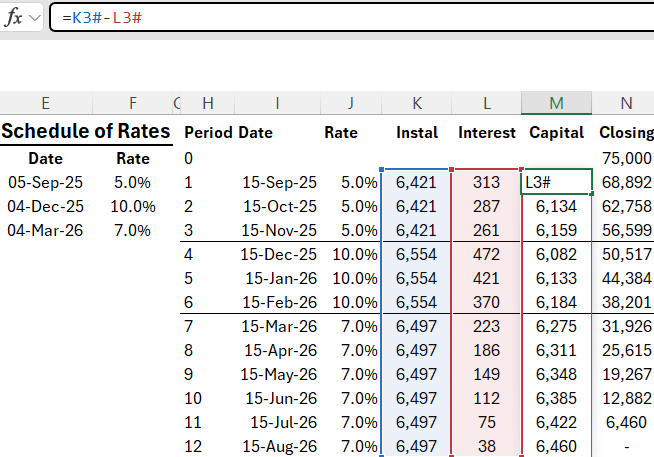
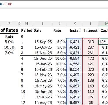
The key to automation lies in converting static formulas into spilling arrays. While the SEQUENCE and EDATE functions already spill automatically, other columns need manual conversion using the # (spill range) operator.

Converting the Rate Column:

Replace fixed cell references with dynamic ranges by adding # after the initial cell reference. When you reference E2# instead of E2, Excel treats the entire spilled range as input. You'll encounter #SPILL! errors initially—this indicates cells are blocking the spill range. Delete these obstructing cells to allow the formula to expand freely.

Applying to Remaining Columns:

Repeat this process for:

• Installment calculations (PMT function)

• Interest portions (IPMT function)

• Principal portions (PPMT function)

Each formula component that references another column should use the # operator. When you extend the loan period from 12 to 24 months, all columns automatically expand without manual intervention.

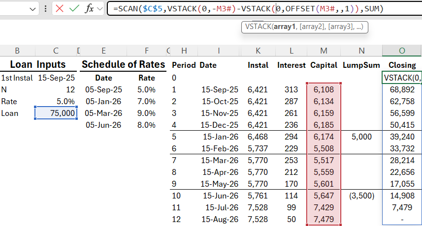
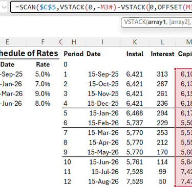
4. Handling Closing Balance Calculations Using SCAN & VSTACK Functions

The closing balance column presents a unique challenge in excel amortization schedule dynamic array formulas because it requires calculating a running total that decreases with each principal payment. Traditional cell-by-cell references won't work in a fully dynamic model.

The SCAN Function for Running Balances

The SCAN function specializes in creating accumulating or decreasing totals across a range. Here's how it works for loan balances:

excel =SCAN(starting_value, array, LAMBDA(accumulator, value, accumulator - value))

Key components:

• Starting value: The initial loan principal (e.g., 75,000)

• Array: The principal repayment column

• Operation: Subtraction to decrease the balance each period

This creates a running balance that automatically adjusts as principal payments change throughout the schedule.

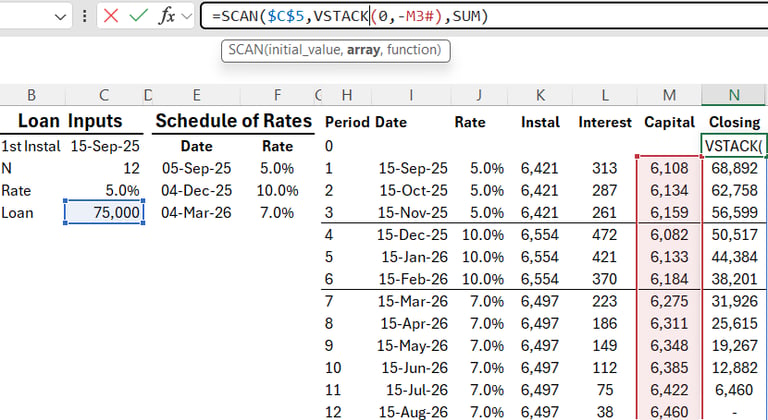
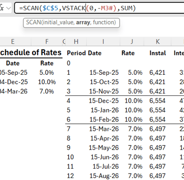
Adding the Initial Balance with VSTACK

The SCAN function alone produces balances starting from period 1. To include the initial principal amount at period 0:

excel =VSTACK(0, SCAN(initial_principal, principal_column#, LAMBDA(a, v, a - v)))

The VSTACK function prepends a zero (representing the opening position) before the SCAN calculation, ensuring the entire balance column aligns perfectly with other columns.

Synchronizing Array Sizes with DROP

When referencing the closing balance in other formulas (interest calculations, installment calculations), the array size must match. Since VSTACK adds one extra row, use the DROP function:

excel =DROP(closing_balance_formula, 1)

This removes the first row, creating a range identical in size to other dynamic columns. This synchronization is essential for advanced excel functions for loan modeling to work seamlessly across all calculations.

5. Adding Balloon Payments and Lump Sum Transactions

Real-world loans often involve irregular transactions beyond standard monthly payments. An excel loan calculator with balloon payment capabilities requires an additional column to track these variations. The dynamic excel loan template with balloon and lump sum functionality transforms a basic amortization schedule into a practical financial tool, such as the one detailed in this guide on creating a loan amortization schedule in Excel.

Setting Up the Lump Sum Column

Insert a new column labeled "Lump Sums" adjacent to your existing amortization table. This column captures:

• Deposits that reduce the outstanding balance

• Withdrawals that increase the loan amount

• Balloon payments at specific intervals

Example entries:

1. Period 3: 5,000 (deposit)

2. Period 7: -3,500 (withdrawal)

Referencing Non-Continuous Data with OFFSET

The challenge lies in referencing a non-continuous column within dynamic formulas. The OFFSET function solves this by creating a continuous reference to discontinuous data:

excel =OFFSET(previous_column, 0, 1)

This formula:

• References the column immediately before the lump sum column

• Shifts zero rows (maintains alignment)

• Moves one column to the right (points to lump sums)

Integrating Lump Sums into Closing Balance

Modify the closing balance calculation by adding a zero at the beginning using VSTACK, matching the structure of your capital repayment array:

excel =VSTACK(0, OFFSET(column_reference, 0, 1))

Feed this adjusted range into your SCAN function alongside the principal payments. The closing balance now automatically adjusts when you enter deposits or withdrawals, maintaining accurate tracking throughout the Dynamic Loan Amortization in Excel: How to Model Changing Rates & Balloon Payments schedule.

6. Enhancing Usability with Conditional Formatting for Interest Rate Changes

When building an advanced loan amortization excel schedule with multiple rate periods, visual clarity becomes essential. Long-term loan schedules spanning months or years can make it challenging to spot exactly when interest rates shift, potentially leading to errors during review or analysis.

Why Visual Identification Matters

Conditional formatting transforms your loan table into an intuitive dashboard where rate changes stand out immediately. This visual layer helps financial analysts, accountants, and loan officers quickly identify critical transition points without scanning through hundreds of rows manually.

Setting Up the Conditional Formatting Rule

The technique involves creating a rule that compares each row's interest rate against the previous period:

1. Select the entire data range of your amortization table

2. Navigate to Conditional Formatting > New Rule

3. Choose "Use a formula to determine which cells to format"

4. Enter a formula that checks: IF(current_rate <> previous_rate, TRUE, FALSE)

5. Add a condition to exclude the first row (where no preceding value exists)

6. Apply your preferred formatting style (border, background color, or bold text)

The formula logic ensures that whenever an installment's rate differs from the period before it, Excel automatically highlights that row. This approach works seamlessly with the XLOOKUP function already powering your rate assignments.

Practical Benefits for Complex Loan Analysis

This visual aid proves invaluable when learning how to build advanced loan schedule in excel models for:

• Quick auditing of multi-rate loan portfolios

• Client presentations where rate transitions need emphasis

• Error detection when rates don't align with expected change dates

• Scenario planning involving multiple rate adjustment simulations

Practical Tips & Next Steps for Scaling Loan Models

The dynamic amortization model you've built can expand beyond a single loan scenario. Advanced excel functions for loan modeling like SEQUENCE, SCAN, and XLOOKUP make it possible to replicate this framework across multiple loans simultaneously.

Scaling Across Multiple Loans

• Create separate worksheets for each loan within the same workbook

• Use identical formula structures on each sheet to maintain consistency

• Reference a master input sheet containing all loan parameters (start dates, principals, rate schedules)

• Apply the same dynamic array formulas to automate loan repayments in excel using sequence and scan across your entire portfolio

Portfolio Consolidation Strategies

For users managing multiple loans, our Excel Loan Portfolio Tool provides a complete automated solution with dashboards, sub-schedules, and multi-loan consolidation.

• Aggregating data from 10, 50, or even 100 individual loans

• Building summary dashboards that pull key metrics from multiple amortization schedules

• Creating portfolio-level views showing total outstanding balances, aggregate interest payments, and combined cash flow projections

  Try the advanced loan portfolio dashboard for Excel.

Conclusion

You now have the complete toolkit for building an advanced loan amortization excel model that handles real-world complexity. This dynamic excel loan template with balloon and lump sum capabilities transforms static spreadsheets into powerful financial analysis tools.

Ready to put these techniques into practice?

• Download the sample template linked in the video description for hands-on experimentation

• Apply the SCAN, VSTACK, and XLOOKUP functions to your existing loan models

• Test different scenarios by adjusting interest rates, periods, and lump sum payments

• Watch how your Dynamic Loan Amortization in Excel: How to Model Changing Rates & Balloon Payments automatically recalculates

The beauty of this approach lies in its flexibility. Whether you're managing personal mortgages, business loans, or client portfolios, these self-adjusting formulas eliminate manual updates and reduce errors.

Take action today: Open Excel, enable iterative calculations, and start building your first dynamic amortization schedule. Your financial modeling skills will reach new heights as you master these advanced techniques.

FAQs (Frequently Asked Questions)

What is dynamic loan amortization in Excel and why is it important for financial modeling?

Dynamic loan amortization in Excel refers to creating a self-adjusting loan repayment schedule that can handle changing interest rates and balloon payments. It's important because it allows financial models to accurately reflect real-world scenarios where interest rates fluctuate and lump sum payments occur, ensuring precise tracking of loan balances over time.

How can I model variable interest rates dynamically in an Excel loan amortization schedule?

To model variable interest rates dynamically, create an interest rate schedule with multiple rate periods and corresponding dates. Use the XLOOKUP function with non-exact match mode to assign the correct interest rate per installment period based on date intervals. The SEQUENCE function helps number periods dynamically, allowing flexible schedules that adjust as rates change.

Which Excel functions are essential for building an advanced loan amortization table with changing rates and balloon payments?

Key Excel functions include SEQUENCE for generating period numbers, EDATE for installment dates, PMT for calculating monthly installments, IPMT and PPMT for separating interest and principal portions, SCAN for running totals of closing balances, VSTACK for managing array data like initial principal amounts, OFFSET for referencing lump sum transactions, and XLOOKUP for dynamic rate assignments.

How do I incorporate balloon payments and lump sum transactions into my Excel loan amortization model?

Add an extra column within the amortization table to record lump sum deposits or withdrawals. Use the OFFSET function to continuously reference these non-continuous lump sum entries within closing balance calculations. Modify your closing balance formulas to integrate these lump sums alongside regular repayments, ensuring accurate balances after such transactions.

What techniques can make my Excel loan schedule fully dynamic and self-adjusting when inputs or periods change?

Enable iterative calculations in Excel to support dynamic arrays and spilled formulas. Apply dynamic array techniques like using the # operator to allow columns such as dates, rates, installments, interest, and principal to automatically expand or contract based on input changes. This removes the need for manual formula adjustments when extending periods or modifying inputs.

How can I enhance usability by visually identifying interest rate changes in a long-term loan schedule?

Set up conditional formatting rules in Excel that highlight rows where the interest rate differs from the previous period. This visual aid helps quickly identify when rates change within complex multi-rate loans, making review and analysis more efficient and reducing errors in interpreting the amortization schedule.